Source: FPGN 2026
Authors: HKUST and ETH Zurich
Goals: Lowest possible latency in in-hardware inference. NOT truly novel for neural networks or LUT native networks, mostly focused on achieving nanosecond scale inference.
Notes.
Different from FPGA because it is LUT native. not the first to invent the concept, main goal is to optimize it heavily for speed.
205x latency reduction compared to FPGA based BNN and 30x higher efficiency than previous LUT native networks.
most FPGA based Neural Networks run an algorithm on top of LUTs within the FPGA. this is inefficient. similar with LUT native methods which largely fine tune algorithmic optimizations. the key insight is transforming FPGA fabric itself into a learnable LUT native neural network for ultra low latency acceleration.
hence, “Ultra-Fast Programmable Gate-based Neural accelerators.”
Training
2 training methods


Differentiable Equality Indicator.
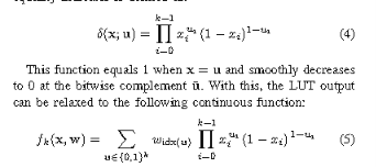
Gradient Attenuation:
2 main issues that cause attenuation:
- repeated multiplications in differentiable equality indicator cause shrink in gradients.
- sigmoid function used for soft binarization narrows effective gradient region
reduced by initializing weights via bimodal distribution using Gaussian distributions applied at the beginning of training.
Design
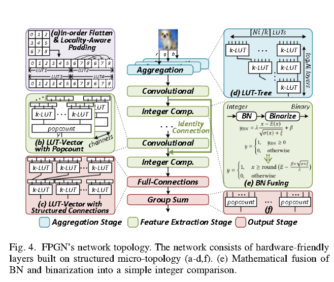
Micro Topological Design.
LUT-Vectors: process input streams in parallel. if multi token inputs, similar to an MoE situation where each LUT is its own expert. provides parallelism and differentiated expertness.
LUT-Tree: input is many binary features but output is supposed to be one binary decision. instead of running all those binary features through every LUT one at a time, it splits the features and then feeds different features to different LUTs then processes the output of those LUTs to a final LUT which gives the binary decision. done in 2 LUT layers here.
Popcount: instead of making a decision, it counts how many features activated. decision from LUT tree may be yes or no, but Popcount may say 4/6 bits activated.
2 rules to how it works:
- In-Order Flattening: flattening high dimensional feature data into ordered bit vector. the order is directly used to determine LUT connections
- Locality Aware Padding: if there are only 4 usable bits instead of 6, 2 bits are repeated so as to not leave an LUT functionally empty.
Macro Topological Design:
Aggregation Stage: reduce info loss and costly floating point preprocessing by using learned pixel wise aggregation layer instead of conventional quantization. it is a convolutional-style layer with a LUT tree as the 1x1 convolutional kernel to convert different input channels into a single informative activation.
Feature Extraction Stage: stack of blocks with LUT-Conv layers implemented as channel wise parallel LUT-Vectors & popcount units. performs k-to-1 mapping within each LUT.
Output Stage: cascaded FC layers and a task specific unit. for classification, the task specific unit implements a popcount-based group sum operation to get final scores with high precision required for robust classification performance.
Fig 1.
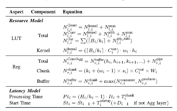
Full Streaming Hardware Architecture:
- Flexible Intra Layer Spatial Computation: to adjust LUT resource utilization under different resource, they use configurable unrolling through kernel-sharing. instead of unrolling 1 position to kernel per cycle, they unroll many in the same cycle
- Adaptive Intra-Layer Pipelining: ensure high freq timing closure, implement an adaptive pipelining strategy within processing units. Intra layer processing units are of 2 kinds—LUT-vectors and popcount reduction units. they add registers at strategic points to break clock cycle into smaller pipelines to maintain high freq.
- LUT-Efficient Inter-Layer Streaming: instead of making layer 2 wait for layer 1 to finish, it works via stationary window circular line where the part within the window is stationary and data is moved along and can be read by layer 2, while layer 1 continues to work outside of it. hence allowing concurrent operation.
Evaluation
QoR key equations:
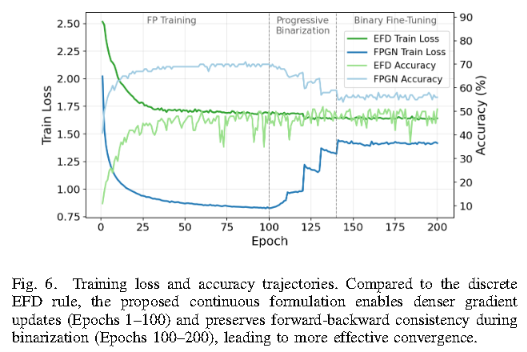
- progressive binarization + binary fine tuning is better than EFD as it converges faster exhibits less fluctuations because current training limits to one entry out of 2^k parameters. maintains lower loss and higher accuracy than EFD.
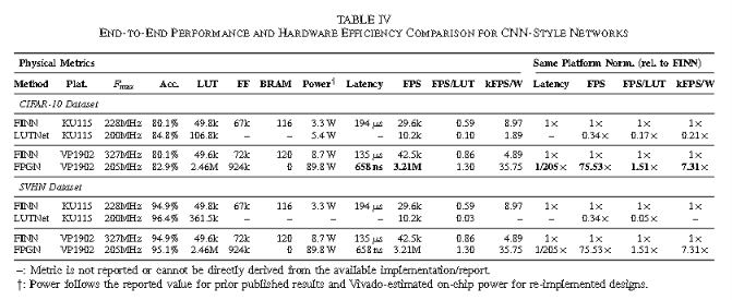
- LUT utilization remains the dominant resource constraint
Notes from the Author.
$email context: robotics MPPI based on FPGN chip
Thanks for you interest. But, since we are not expertise of robotic, we cannot answer your question in detal. After discussion, we can only give you some, maybe useful, comments:
FPGN is design to NNs. Though we evaluate CNN-style network here, it can also be used to build Transformer and RNN, which might be useful to “continuous-valued state-transition prediction and repeated multi-step rollouts” you mentioned. You can refer to these two papers: LL-ViT: Edge Deployable Vision Transformers with Look Up Table Neurons; Recurrent Deep Differentiable Logic Gate Networks
If your target is a huge NN model, the resource and routing are the most critical problems. I suggests a model with small size. In fact, I think the most suitable domain for FPGN, and even for all LUT-as-neuron paradigm, is some simple but latency sensitive tasks, such as jet and kws, that are simple but require ~ns latency.
BRs, Jiawei
$email context: surrogate gradients for fine tuning
During the binary fine-tuning stage, binary computing is used in forward and floating gradient is calculated during backward, the same to prior stages. So, the gradient surrogate is already used.
BRs, Jiawei